Report Gilberto Quintos
Abstract Machine learning use has grown tremendously in the past ten years. Machine learning concepts are paving the way for a new era of daily life with the use of machine learning in places such as the automotive industry, bioinformatics industry, gaming industry along with just about every industry. This paper will briefly review the advances in machine learning and also go in depth of three papers that used machine learning to solve important complex problems.
Machine learning has grown in popularity since 1997 when IBM’s Deep Blue beat a World Champion Chess Player. Deep learning in particular has grown substantially since 2012 when the paper AlexNet[1] was published. Since then many more network architectures have been published building off the idea of AlexNet such as VGG Net[2], RESNet[3], DenseNet[4],and the Fully Convolutional Network(FCN)[5]. Some of these network architectures have then been even further expanded on such as in “A Joint Convolutional Neural Networks and Context Transfer for Street Scenes Labeling”[6] and “Embedding Structured Contour and Location Prior in Siamesed Fully Convolutional Networks for Road Detection”[7]. There have also been attempts to use machine learning in network security such as “Deep Learning Approach for Network Intrusion Detection in Software Defined Networking”[8] and “Machine learning classification over encrypted data”[9]. A field I am interested in to see machine learning be of use would be the media compression field but as the paper “Machine learning for media compression: challenges and opportunities”[10] the field of media compression is not well suited for machine learning concepts.
The rest of this report will be summarizing three papers that are related to the topics talked about in class while also giving my own brief opinion on each of the three papers. These are the following papers: Atom Net[11] Pafnucy[12] Alphago[13]
These three papers involve machine learning techniques to solve multiple problems. The first two papers are dealing with using machine learning to attempt to solve problems in chemistry and the last paper is a breakthrough in AI using machine learning and other techniques to master the game of Go. The end of this report will also be describing a commonality found within these three papers that may be of use when attempting other tasks in machine learning. AtomNet: A Deep Convolutional Neural Network for Bioactivity Prediction in Structure-based Drug Discovery This paper was published on October, 10, 2015 and the authors are Izhar Wallach, Michael Dzamba, and Abraham Heifets. These three people all work for Atomwise a company formed in 2012 to use artificial intelligence to help discover new medicines. This paper aims to “predict the bioactivity of small molecules for drug discovery applications” using deep neural networks. They introduce the use of a classical convolutional neural network architecture which they coin as, AtomNet, to help address the challenge of accurately predicting molecular binding of the physical interaction of molecules. The paper describes research in this topic to be able to “reduce the time-to-discovery of new treatments,” and “help eliminate toxic molecules early in development, and guide medicinal chemistry efforts”. They argue deep convolutional neural networks(DCNN) “leverage the spatial and temporal structure of its domain” , also ,“local low-level features are then hierarchically composed by the network into larger, more complex features (e.g., for a face recognition task, pixels may be combined into edges; edges into eyes and noses; eyes and noses into faces)”. They argue since chemical groups are defined by their spatial arrangement and bonding of multiple atoms in space that are proximate to each other and thus the strength of DCNN to achieve high accuracy for structure-based binding affinity prediction. To implement such a theory they obtain a pre-made dataset, the Directory of Useful Decoys Enhance(DUDE)[14], a self-made dataset they called ChEMBL-20 PMD, and another dataset with only Experimentally verified inactives. These three datasets can be broadly described as having three parts. Targets Actives Decoys Each dataset has a total amount of targets,actives,and decoys. For example the DUDE dataset has a total of 102 targets, 22,886 actives(average of 224 active per target), and 50 decoys per active(hence around 1,144,300 decoys in total). The target is a molecular compound such as Androgen Receptor, FK506-binding protein 1A, and other such compounds. The actives are target specific molecular compounds that are known to or highly likely to bind to the target. The decoys are target specific molecular compounds known to or highly likely to not bind to the target. As such the goal would be to accurately predict if a certain active or decoy would bind to a target. Thus such a system would also be able to predict with high confidence if a never before seen target and a never before seen active or decoy bind or not. Having a high confidence if an active or decoy bind to a target can significantly speed up the drug trial process. The DCNN is made up of 3D convolutional layers with an architecture of “four convolutional layers of 128×53, 256×33, 256×33, 256×33(number of filters × filter-dimension), and two fully-connected layers with 1024 hidden units each, topped by a logistic-regression cost layer over two activity classes.”. The input layer receives vectorized versions of 1 Angstrom 3D grids placed over co-complexes of the target proteins and small-molecules that are sampled within the target’s binding site. First, they define the binding site using a flooding algorithm seeded by a bound active. Second, they shift the coordinate of the co-complexes to a 3D Cartesian system originated at the center-of-mass of the binding site. Third, they sample multiple poses within the binding site cavity. Fourth, they crop the geometric data to fit within an appropriate bounding box. In the study they used a cube of 20 Angstroms, centered at the origin. Fifth, they translate the input data into a fixed-size grid with 1 Angstrom spacing. Each grid cell holds a value that represents the presence of some basic structural features in that location. Basic structural features can vary from a simple enumeration of atom types to more complex protein-ligand descriptors such as interaction fingerprints of the target and bound active/decoy. Lastly, they unfold the 3D grid into a 1D floating point vector
The results are as follows:
 Table 1: Comparisons of AtomNet and Smina on the DUDE, ChEMBL-20-PMD, and ChEMBL-20 inactives benchmarks. DUDE-30 refers to the held-out set of 30 targets whereas DUDE-102 refers to the full dataset.
“On each of our four evaluation data sets, AtomNet achieves an order-of-magnitude improvement over Smina at a level of accuracy useful for drug discovery” As can be seen from the results using the DCNN’s strength of finding patterns in local low-level features lends itself well to be used on 3D structured data of molecular compounds.
Development and evaluation of a deep learning model for protein–ligand
binding affinity prediction
This paper was Received on January 3, 2018; revised on March 30, 2018; editorial decision on April 30, 2018; accepted on May 4, 2018 and has advance access publication date of: 10 May 2018 and the authors are Marta M.Stepniewska-Dziubinska, Piotr Zielenkiewicz, Pawel Siedlecki. These three people work at the Institute of Biochemistry and Biophysics and Department of Systems Biology, Institute of Experimental Plant Biology and Biotechnology, University of Warsaw. This paper similar to the last one also attempts structure based ligand discovery using machine learning methodologies.They use a deep neural network which they coin, Pafnucy (pronounced ‘paphnusy’), to also attempt structure based ligand discovery. The network architecture can be seen below:
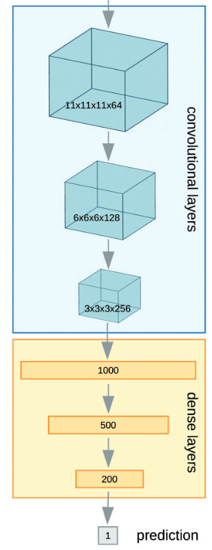 As can be seen the neural network is composed of two parts which should be fairly evident. The first part is the convolutional layers(blue) of the network while the second part is the fully connected or dense layers part of the network. The last part is the prediction layer which predicts the binding affinity of the input.
‘Pafnucy uses 3 convolutional layers with 64, 128 and 256 filters. Each layer has 5-Ångstrom cubic filters and is followed by a max pooling layer with a 2-Ångstrom cubic patch. The result of the last convolutional layer is flattened and used as input for a block of dense (fully-connected) layers. They used 3 dense layers with 1000, 500 and 200 neurons. In order to improve generalization, dropout with drop probability of 0.5 was used for all dense layers… Both convolutional and dense layers are composed of rectified linear units (ReLU).’
As seen the Pafnucy network is a rather simple network with the size of the filters of 5 Angstrom chosen to in theory help the network find local interactions between atoms in close proximity.
The network architecture though is not something that is particularly unique. The part that is different is the way the data is prepared and presented to the network. They cropped the complex to a
defined size of 20-Å cubic box focused at the geometric center of a ligand. They then discretized the positions of heavy atoms using a 3D grid with 1-Å resolution.
In Pafnucy, 19 features were used to describe an atom:
9 bits(one-hot or all null) encoding atom types: B,C,N,O,P,S,Se,halogen and metal
1 integer (1,2,or 3) with atom hybridization: hyb
1 integer counting the numbers of bonds with other heavyatoms: heavy_valence
1 integer counting the number of bonds with other heteroatoms: hetro_valence
5 bits (1 if present) encoding properties defined with SMARTS patterns: hydrophobic, aromatic, acceptor,donor,ring
1 float with partial charge: partialcharge
1 integer (1 for ligand, -1 for protein) to distinguish between the two molecules: moltype
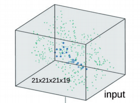
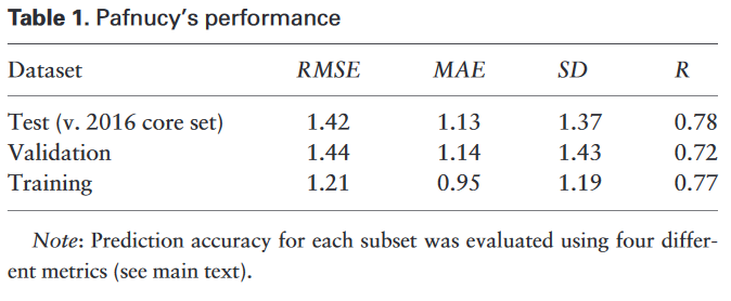
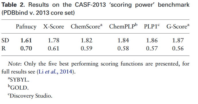 Each of the above features were placed in their own 3D cube then stacked to create a 21x21x21x19 data structure. So for example if you would like to know if the atom at position [0,0,0] of the 3D data was that of a ligand atom or protein atom you would check the last cube in the stack since the last 3D cube is used to distinguish between the two types. If you would like to know if the atom at position [0,0,0] was a metal you would look at the ninth cube in the stack since the first nine cubes in the stack represent the following atom types: B,C,N,O,P,S,Se,halogen and metal.
The results can be seen above:
To their knowledge,the only scoring function with better performance published so far is
RF-Score v3, which achieves R = 0.74 and SD = 1.51 on CASF-2013.
One interesting note is that they were able to see which features used in the data the Pafnucy network found to be better by looking at the change of the weight the network had after training.
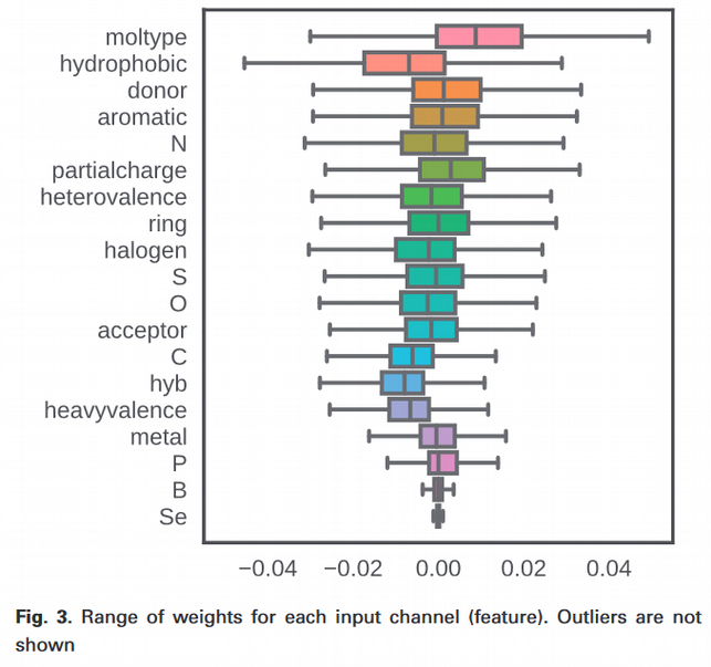 As can be seen from the image to the left the Pafnucy network found the best way to achieve its results to be dictated by the moltype of the atoms followed by the hydrophobic property of the atoms. As can be seen the least discriminative feature was the atom type Se. As the authors carefully point out though this does not mean the atom type Se can not be used to provide accurate binding affinity values, simply that the network judged the atom type to not be discriminative enough compared to the other features, hence gave greater weights to the other features
The results show the Pafnucy network can provide state of the art performance while being simple in design and autonomous in nature.
Mastering the game of Go with deep neural networks and tree search
This paper has 20 authors all from a company called Deepmind which was bought by Google. This papers goal was to master the game of Go and in doing so propelled the state of AI.
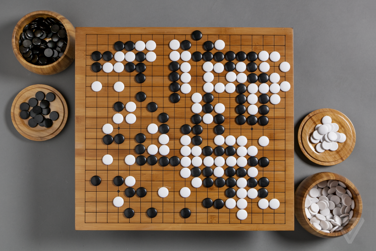 Go is a game that originated in China that is said to be the most complicated board game. The total number of possible games of Go has been estimated at 1076. The entire universe is estimated to contain “only” about 1080 atoms.
In 1997, Garry Kasparov was defeated by Deep Blue, a computer program written by IBM, running on a supercomputer. This was the first time that a reigning world chess champion was defeated by a computer program in tournament conditions. Both AlphaGo and Deep Blue represent their respective game in a structure called a game tree. A game tree represents states of the game as nodes in the tree. The tree can be explained by the root representing the beginning of the game while the first branches from the root represent every possible move from the the root. The second layer would constitute every possible move for the second move of the game from every possible previous move and so on. The number of nodes of such a tree when pertaining to chess has estimated to be 10120 nodes which is impossible to store on a computer let alone compute on it. Deep Blue solved this problem by only searching around six moves ahead of the current game state and also using a huerstic on the searched moves to be able to choose a single move effectively and efficiently.
AlphaGo solved this problem by using a different approach made up of three distinct and parts in tandem:
- Value network a. Provides overall position judgment
- Monte Carlo Tree Search (MCTS) algorithm
- Policy network(Split into three parts)
a. Supervised-learning move picker(mimic human moves)
b. Reinforced-learning move picker
c. Quick move picker
Firstly the MCTS can be described as such “The focus of Monte Carlo tree search is on the analysis of the most promising moves, expanding the search tree based on random sampling of the search space. The application of Monte Carlo tree search in games is based on many playouts. In each playout, the game is played out to the very end by selecting moves at random. The final game result of each playout is then used to weight the nodes in the game tree so that better nodes are more likely to be chosen in future playouts. ”[15].
Secondly the value network takes an input of a representation of the current game state and gives an over probability of winning. The architecture is as follows
The first hidden layer zero pads the input into a 23×23 image, then convolves 128 filters(depth) of kernel size 5×5(window size) with stride 1(how much the window moves after one convolution) with Relu activation function.
Hidden layers 2 to 12 zero pads the respective previous hidden layer into a 21×21 image, then convolves 128 filters of kernel size 3×3 with stride 1 with Relu activation function.
Hidden layer 13 convolves 1 filter of kernel size 1×1 with stride 1 with Relu activation function.
Hidden layer 14 is a fully connected linear layer with 256 rectifier units.
Output layer is a fully connected linear layer with a single tanh unit. The value network architecture is very deep with multiple convolutions and sine the policy network is rather similar I will skip the architecture for those networks.
Lastly they trained two policy networks. The first network attempts to predict the next move to be made by the opponent on the entire board and the second policy network only attempts to predict the opponent’s next move in a local region of the board.
They use these three neural networks and MCTS in tandem to supplement the heuristic and game tree that Deep Blue used.
The data used to train the networks are as follows:
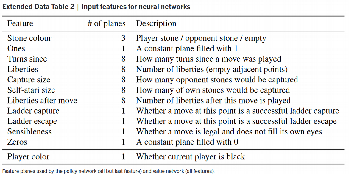 As seen each feature plane is a 19x19 2D matrix since the Go board is a 19x19 board stacked on top of each other to make a 3D cube of size 19x19x48 for the policy networks and 19x19x49 for the value network. Each feature in the planes was chosen in order to emphasize certain game rules or to help the networks determine the optimal prediction for winning the game.
The results of this work were plainly seen on March 9-15 2016 when AlphaGo beat Lee Sedol a world renowned Go competitor in a 5 game match with 4 wins and one loss.
The common thread that I discovered might be well known to people who understand machine learning more fundamentally but to me was something new that I managed to understand. The common theme in these three papers to me seems to be the concept of identifying important features from the problem set and then stacking them into a data structure to then use convolutions on them. For example the first paper though you only needed structured molecule data in 3D-space hence only used a single cube to represent data. The second paper took this further and identified 19 3D features they deemed important and stacked each of these 3D structured data into a 21x21x21x19 data structure. AlphaGo found 49 2D features they deemed important and stacked them to create a 3D cube of size 19x19x49. They then each used either 3D convolutions if patterns in space mattered,such as the first two papers, or 2D convolutions if patterns in 2D space mattered, such as the AlphaGo paper. You could extrapolate this pattern of data structuring to any problem with proper data and properly chosen features.
References [1] : Krizhevsky, A., Sutskever, I., and Hinton, G. E. ImageNet classification with deep convolutional neural networks. In NIPS, pp. 1106–1114, 2012. [2] : Simonyan, Karen, and Andrew Zisserman. “Very deep convolutional networks for large-scale image recognition.” arXiv preprint arXiv:1409.1556 (2014). [3] : He, Kaiming, et al. “Deep residual learning for image recognition.” Proceedings of the IEEE conference on computer vision and pattern recognition. 2016. [4] : Huang, Gao, et al. “Densely connected convolutional networks.” CVPR. Vol. 1. No. 2. 2017. [5] : Long, Jonathan, Evan Shelhamer, and Trevor Darrell. “Fully convolutional networks for semantic segmentation.” Proceedings of the IEEE conference on computer vision and pattern recognition. 2015. [6] : Wang, Qi, Junyu Gao, and Yuan Yuan. “A joint convolutional neural networks and context transfer for street scenes labeling.” IEEE Transactions on Intelligent Transportation Systems 19.5 (2018): 1457-1470. [7] : Wang, Qi, Junyu Gao, and Yuan Yuan. “Embedding structured contour and location prior in siamesed fully convolutional networks for road detection.” IEEE Transactions on Intelligent Transportation Systems 19.1 (2018): 230-241. [8] : Tang, Tuan A., et al. “Deep learning approach for network intrusion detection in software defined networking.” Wireless Networks and Mobile Communications (WINCOM), 2016 International Conference on. IEEE, 2016. [9] : Bost, Raphael, et al. “Machine learning classification over encrypted data.” NDSS. 2015. [10] : Said, Amir. “Machine learning for media compression: challenges and opportunities.” APSIPA Transactions on Signal and Information Processing 7 (2018). [11] : Wallach, Izhar, Michael Dzamba, and Abraham Heifets. “AtomNet: A deep convolutional neural network for bioactivity prediction in structure-based drug discovery.” arXiv preprint arXiv:1510.02855 (2015). [12] : Marta M Stepniewska-Dziubinska, Piotr Zielenkiewicz, Pawel Siedlecki; Development and evaluation of a deep learning model for protein–ligand binding affinity prediction, Bioinformatics, Volume 34, Issue 21, 1 November 2018, Pages 3666–3674, https://doi.org/10.1093/bioinformatics/bty374 [13] : Silver, David, et al. “Mastering the game of Go with deep neural networks and tree search.” nature 529.7587 (2016): 484. [14] : M. M. Mysinger, M. Carchia, J. J. Irwin, and B. K. Shoichet, “Directory of useful decoys, enhanced (dud-e): Better ligands and decoys for better benchmarking,”Journal of Medicinal Chemistry, vol. 55, no. 14, pp. 6582–6594, 2012. PMID: 22716043. [15] : https://en.wikipedia.org/wiki/Monte_Carlo_tree_search